Pliocene

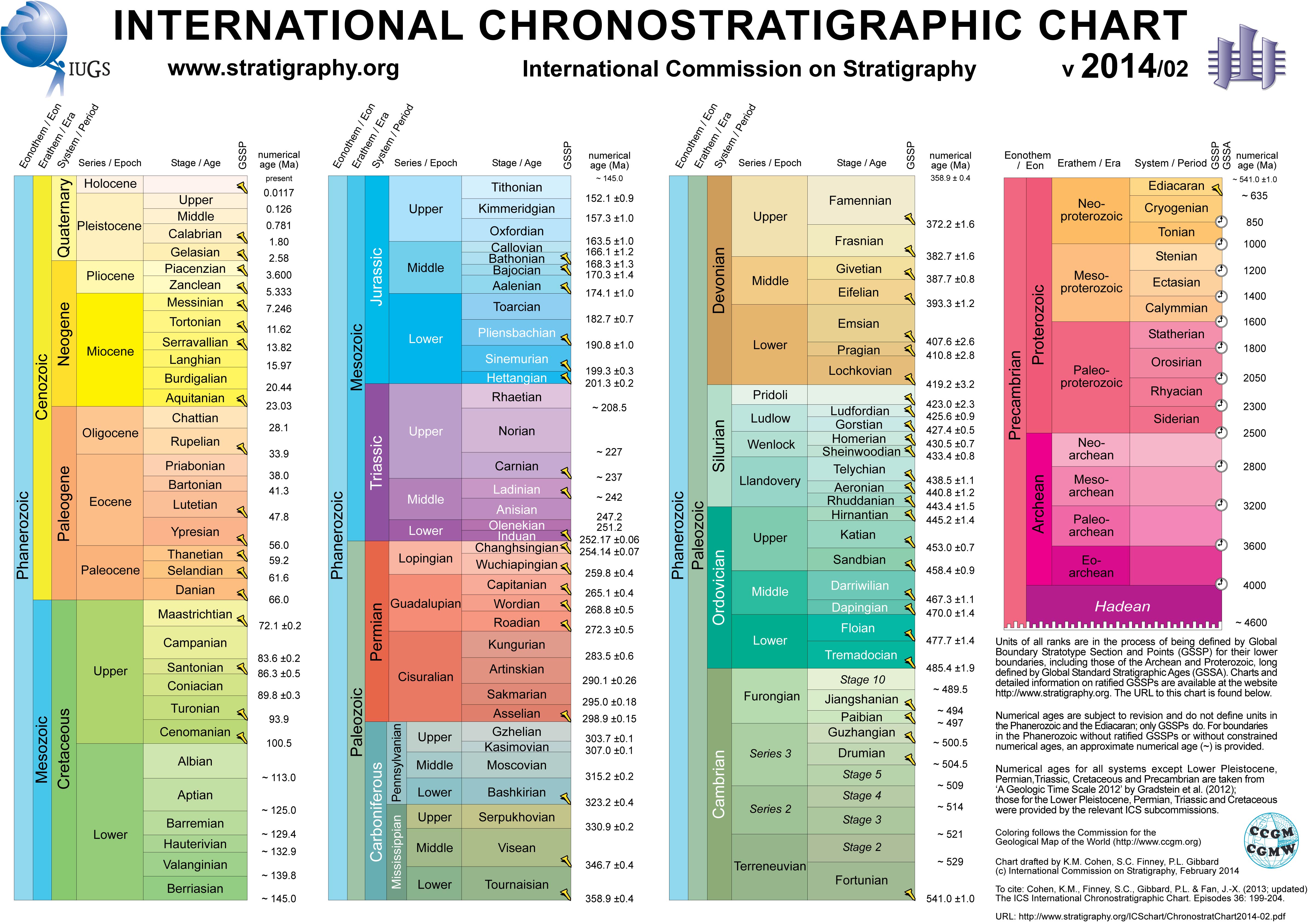
The Pliocene (Template:IPAc-en Template:Respell;Template:RefnTemplate:Refn also Pleiocene)Template:Refn is the epoch in the geologic time scale that extends from 5.33 to 2.58 million years ago (Ma). It is the second and most recent epoch of the Neogene Period in the Cenozoic Era. The Pliocene follows the Miocene Epoch and is followed by the Pleistocene Epoch. Prior to the 2009 revision of the geologic time scale, which placed the four most recent major glaciations entirely within the Pleistocene, the Pliocene also included the Gelasian Stage, which lasted from 2.59 to 1.81 Ma, and is now included in the Pleistocene. The name comes from Ancient Greek πλείων (pleíōn), meaning "most", and καινός (kainós), meaning "new, recent".

As with other older geologic periods, the geological strata that define the start and end are well-identified but the exact dates of the start and end of the epoch are slightly uncertain. The boundaries defining the Pliocene are not set at an easily identified worldwide event but rather at regional boundaries between the warmer Miocene and the relatively cooler Pleistocene. The upper boundary was set at the start of the Pleistocene glaciations.

Etymology

Charles Lyell (later Sir Charles) gave the Pliocene its name in Principles of Geology (volume 3, 1833).

The name "Pliocene" comes from Ancient Greek πλείων (pleíōn), meaning "most", and καινός (kainós), meaning "new", and means roughly "continuation of the recent", referring to the essentially modern marine mollusc fauna.

Subdivisions

File:Pliocene Chart.jpg

Some schemes for subdivisions of the Pliocene

In the official timescale of the ICS, the Pliocene is subdivided into two stages. From youngest to oldest they are:

• Piacenzian (3.60–2.58 Ma)
• Zanclean (5.33–3.60 Ma)

The Piacenzian is sometimes referred to as the Late Pliocene, whereas the Zanclean is referred to as the Early Pliocene.

In the system of

• North American Land Mammal Ages (NALMA) include Hemphillian (9–4.75 Ma), and Blancan (4.75–1.6 Ma). The Blancan extends forward into the Pleistocene.
• South American Land Mammal Ages (SALMA) include Montehermosan (6.8–4.0 Ma), Chapadmalalan (4.0–3.0 Ma) and Uquian (3.0–1.2 Ma).

In the Paratethys area (central Europe and parts of western Asia) the Pliocene contains the Dacian (roughly equal to the Zanclean) and Romanian (roughly equal to the Piacenzian and Gelasian together) stages. As usual in stratigraphy, there are many other regional and local subdivisions in use.

In Britain, the Pliocene is divided into the following stages (old to young): Gedgravian, Waltonian, Pre-Ludhamian, Ludhamian, Thurnian, Bramertonian or Antian, Pre-Pastonian or Baventian, Pastonian and Beestonian. In the Netherlands the Pliocene is divided into these stages (old to young): Brunssumian C, Reuverian A, Reuverian B, Reuverian C, Praetiglian, Tiglian A, Tiglian B, Tiglian C1-4b, Tiglian C4c, Tiglian C5, Tiglian C6 and Eburonian. The exact correlations between these local stages and the International Commission on Stratigraphy (ICS) stages is not established.

Climate

File:Pliocene sst anomaly.png

Mid-Pliocene reconstructed annual sea surface temperature anomaly

During the Pliocene epoch (5.3 to 2.6 million years ago (Ma)), the Earth's climate became cooler and drier, as well as more seasonal, marking a transition between the relatively warm Miocene to the cooler Pleistocene. However, the beginning of the Pliocene was marked by an increase in global temperatures relative to the cooler Messinian. This increase was related to the 1.2 million year obliquity amplitude modulation cycle. By 3.3–3.0 Ma, during the Mid-Piacenzian Warm Period (mPWP), global average temperature was 2–3 °C higher than today, while carbon dioxide levels were the same as today (400 ppm). Global sea level was about 25 m higher, though its exact value is uncertain. The northern hemisphere ice sheet was ephemeral before the onset of extensive glaciation over Greenland that occurred in the late Pliocene around 3 Ma. The formation of an Arctic ice cap is signaled by an abrupt shift in oxygen isotope ratios and ice-rafted cobbles in the North Atlantic and North Pacific Ocean beds. Mid-latitude glaciation was probably underway before the end of the epoch. The global cooling that occurred during the Pliocene may have accelerated on the disappearance of forests and the spread of grasslands and savannas.

During the Pliocene the earth climate system response shifted from a period of high frequency-low amplitude oscillation dominated by the 41,000-year period of Earth's obliquity to one of low-frequency, high-amplitude oscillation dominated by the 100,000-year period of the orbital eccentricity characteristic of the Pleistocene glacial-interglacial cycles.

During the late Pliocene and early Pleistocene, 3.6 to 2.6 Ma, the Arctic was much warmer than it is at the present day (with summer temperatures some 8 °C warmer than today). That is a key finding of research into a lake-sediment core obtained in Eastern Siberia, which is of exceptional importance because it has provided the longest continuous late Cenozoic land-based sedimentary record thus far.

During the late Zanclean, Italy remained relatively warm and humid. Central Asia became more seasonal during the Pliocene, with colder, drier winters and wetter summers, which contributed to an increase in the abundance of Template:C4 plants across the region. In the Loess Plateau, δ13C values of occluded organic matter increased by 2.5% while those of pedogenic carbonate increased by 5% over the course of the Late Miocene and Pliocene, indicating increased aridification. Further aridification of Central Asia was caused by the development of Northern Hemisphere glaciation during the Late Pliocene. A sediment core from the northern South China Sea shows an increase in dust storm activity during the middle Pliocene. The South Asian Summer Monsoon (SASM) increased in intensity after 2.95 Ma, likely because of enhanced cross-equatorial pressure caused by the reorganisation of the Indonesian Throughflow.

In the south-central Andes, an arid period occurred from 6.1 to 5.2 Ma, with another occurring from 3.6 to 3.3 Ma. These arid periods are coincident with global cold periods, during which the position of the Southern Hemisphere westerlies shifted northward and disrupted the South American Low Level Jet, which brings moisture to southeastern South America.

From around 3.8 Ma to about 3.3 Ma, North Africa experienced an extended humid period. In northwestern Africa, tropical forests extended up to Cape Blanc during the Zanclean until around 3.5 Ma. During the Piacenzian, from about 3.5 to 2.6 Ma, the region was forested at irregular intervals and contained a significant Saharan palaeoriver until 3.35 Ma, when trade winds began to dominate over fluvial transport of pollen. Around 3.26 Ma, a strong aridification event that was followed by a return to more humid conditions, which was itself followed by another aridification around 2.7 Ma. From 2.6 to 2.4 Ma, vegetation zones began repeatedly shifting latitudinally in response to glacial-interglacial cycles.

The climate of eastern Africa was very similar to what it is today. Unexpectedly, the expansion of grasslands in eastern Africa during this epoch appears to have been decoupled from aridification and not caused by it, as evidenced by their asynchrony.

Southwestern Australia hosted heathlands, shrublands, and woodlands with a greater species diversity compared to today during the Middle and Late Pliocene. Three different aridification events occurred around 2.90, 2.59, and 2.56 Ma, and may have been linked to the onset of continental glaciation in the Arctic, suggesting that vegetation changes in Australia during the Pliocene behaved similarly to during the Late Pleistocene and were likely characterised by comparable cycles of aridity and humidity.

The equatorial Pacific Ocean sea surface temperature gradient was considerably lower than it is today. Mean sea surface temperatures in the east were substantially warmer than today but similar in the west. This condition has been described as a permanent El Niño state, or "El Padre". Several mechanisms have been proposed for this pattern, including increased tropical cyclone activity.

The extent of the West Antarctic Ice Sheet oscillated at the 40 kyr period of Earth's obliquity. Ice sheet collapse occurred when the global average temperature was 3 °C warmer than today and carbon dioxide concentration was at 400 ppmv. This resulted in open waters in the Ross Sea. Global sea-level fluctuation associated with ice-sheet collapse was probably up to 7 meters for the west Antarctic and 3 meters for the east Antarctic. Model simulations are consistent with reconstructed ice-sheet oscillations and suggest a progression from a smaller to a larger West Antarctic ice sheet in the last 5 million years. Intervals of ice sheet collapse were much more common in the early-mid Pliocene (5 Ma – 3 Ma), after three-million-year intervals with modern or glacial ice volume became longer and collapse occurs only at times when warmer global temperature coincide with strong austral summer insolation anomalies.

Paleogeography

File:Great American Biotic Interchange examples.svg

Examples of migrant species in the Americas after the formation of the Isthmus of Panama. Olive green silhouettes denote North American species with South American ancestors; blue silhouettes denote South American species of North American origin.

Continents continued to drift, moving from positions possibly as far as 250 km from their present locations to positions only 70 km from their current locations. South America became linked to North America through the Isthmus of Panama during the Pliocene, making possible the Great American Interchange and bringing a nearly complete end to South America's distinctive native ungulate fauna, though other South American lineages like its predatory mammals were already extinct by this point and others like xenarthrans continued to do well afterwards. The formation of the Isthmus had major consequences on global temperatures, since warm equatorial ocean currents were cut off and an Atlantic cooling cycle began, with cold Arctic and Antarctic waters decreasing temperatures in the now-separated Atlantic Ocean.

Africa's collision with Europe formed the Mediterranean Sea, cutting off the remnants of the Tethys Ocean. The border between the Miocene and the Pliocene is also the time of the Messinian salinity crisis.

During the Late Pliocene, the Himalayas became less active in their uplift, as evidenced by sedimentation changes in the Bengal Fan.

The land bridge between Alaska and Siberia (Beringia) was first flooded near the start of the Pliocene, allowing marine organisms to spread between the Arctic and Pacific Oceans. The bridge would continue to be periodically flooded and restored thereafter.

Pliocene marine formations are exposed in northeast Spain, southern California, New Zealand, and Italy.

During the Pliocene parts of southern Norway and southern Sweden that had been near sea level rose. In Norway this rise elevated the Hardangervidda plateau to 1200 m in the Early Pliocene. In Southern Sweden similar movements elevated the South Swedish highlands leading to a deflection of the ancient Eridanos river from its original path across south-central Sweden into a course south of Sweden.

Environment and evolution of human ancestors

The Pliocene is bookended by two significant events in the evolution of human ancestors. The first is the appearance of the hominin Australopithecus anamensis in the early Pliocene, around 4.2 million years ago. The second is the appearance of Homo, the genus that includes modern humans and their closest extinct relatives, near the end of the Pliocene at 2.6 million years ago. Key traits that evolved among hominins during the Pliocene include terrestrial bipedality and, by the end of the Pliocene, encephalized brains (brains with a large neocortex relative to body massTemplate:Efn and stone tool manufacture.

Improvements in dating methods and in the use of climate proxies have provided scientists with the means to test hypotheses of the evolution of human ancestors. Early hypotheses of the evolution of human traits emphasized the selective pressures produced by particular habitats. For example, many scientists have long favored the savannah hypothesis. This proposes that the evolution of terrestrial bipedality and other traits was an adaptive response to Pliocene climate change that transformed forests into more open savannah. This was championed by Grafton Elliot Smith in his 1924 book, The Evolution of Man, as "the unknown world beyond the trees", and was further elaborated by Raymond Dart as the killer ape theory. Other scientists, such as Sherwood L. Washburn, emphasized an intrinsic model of hominin evolution. According to this model, early evolutionary developments triggered later developments. The model placed little emphasis on the surrounding environment. Anthropologists tended to focus on intrinsic models while geologists and vertebrate paleontologists tended to put greater emphasis on habitats.Template:Sfn

Alternatives to the savanna hypothesis include the woodland/forest hypothesis, which emphasizes the evolution of hominins in closed habitats, or hypotheses emphasizing the influence of colder habitats at higher latitudes or the influence of seasonal variation. More recent research has emphasized the variability selection hypothesis, which proposes that variability in climate fostered development of hominin traits. Improved climate proxies show that the Pliocene climate of east Africa was highly variable, suggesting that adaptability to varying conditions was more important in driving hominin evolution than the steady pressure of a particular habitat.

Flora

The change to a cooler, drier, more seasonal climate had considerable impacts on Pliocene vegetation, reducing tropical species worldwide. Deciduous forests proliferated, coniferous forests and tundra covered much of the north, and grasslands spread on all continents (except Antarctica). Eastern Africa in particular saw a huge expansion of C₄ grasslands. Tropical forests were limited to a tight band around the equator, and in addition to dry savannahs, deserts appeared in Asia and Africa.

Fauna

Both marine and continental faunas were essentially modern, although continental faunas were a bit more primitive than today.

The land mass collisions meant great migration and mixing of previously isolated species, such as in the Great American Interchange. Herbivores got bigger, as did specialized predators.

Image gallery

• The gastropod Oliva sayana, from the Pliocene of Florida
  The gastropod Oliva sayana, from the Pliocene of Florida
• The coral Cladocora from the Pliocene of Cyprus
  The coral Cladocora from the Pliocene of Cyprus
• A gastropod and attached serpulid wormtube from the Pliocene of Cyprus
  A gastropod and attached serpulid wormtube from the Pliocene of Cyprus
• The gastropod Turritella carinata from the Pliocene of Cyprus
  The gastropod Turritella carinata from the Pliocene of Cyprus
• The thorny oyster Spondylus right and left valve interiors from the Pliocene of Cyprus
  The thorny oyster Spondylus right and left valve interiors from the Pliocene of Cyprus
• The limpet Diodora italica from the Pliocene of Cyprus
  The limpet Diodora italica from the Pliocene of Cyprus
• The scaphopod Dentalium from the Pliocene of Cyprus
  The scaphopod Dentalium from the Pliocene of Cyprus
• The gastropod Aporrhais from the Pliocene of Cyprus
  The gastropod Aporrhais from the Pliocene of Cyprus
• The arcid bivalve Anadara from the Pliocene of Cyprus
  The arcid bivalve Anadara from the Pliocene of Cyprus
• The pectenid bivalve Ammusium cristatum from the Pliocene of Cyprus
  The pectenid bivalve Ammusium cristatum from the Pliocene of Cyprus
• Vermetid gastropod Petaloconchus intortus attached to a branch of the coral Cladocora from the Pliocene of Cyprus
  Vermetid gastropod Petaloconchus intortus attached to a branch of the coral Cladocora from the Pliocene of Cyprus
• Chesapecten, barnacles and sponge borings (Entobia) from the Pliocene of York River, Virginia
  Chesapecten, barnacles and sponge borings (Entobia) from the Pliocene of York River, Virginia

Mammals

File:Landscape of the Pliocene epoch - showing environment at the time of men's appearance - drawn by Riou.jpg

Nineteenth-century artist's impression of a Pliocene landscape

In North America, rodents, large mastodons and gomphotheres, and opossums continued successfully, while hoofed animals (ungulates) declined, with camel, deer, and horse all seeing populations recede. Three-toed horses (Nannippus), oreodonts, protoceratids, and chalicotheres became extinct. Borophagine dogs and Agriotherium became extinct, but other carnivores including the weasel family diversified, and dogs and short-faced bears did well. Ground sloths, huge glyptodonts, and armadillos came north with the formation of the Isthmus of Panama. The latitudinal diversity gradient among terrestrial North American mammals became established during this epoch some time after 4 Ma.

In Eurasia rodents did well, while primate distribution declined. Elephants, gomphotheres and stegodonts were successful in Asia (the largest land mammals of the Pliocene were such proboscideans as Deinotherium, Anancus, and Mammut borsoni,) though proboscidean diversity declined significantly during the Late Pliocene. Hyraxes migrated north from Africa. Horse diversity declined, while tapirs and rhinos did fairly well. Bovines and antelopes were successful; some camel species crossed into Asia from North America. Hyenas and early saber-toothed cats appeared, joining other predators including dogs, bears, and weasels. Template:Human evolution during the Pliocene

In Africa, climatic variability played little role in mammalian extinction and speciation rates. Africa was dominated by hoofed animals, and primates continued their evolution, with australopithecines (some of the first hominins) and baboon-like monkeys such as the Dinopithecus appearing in the late Pliocene. Rodents were successful, and elephant populations increased. Cows and antelopes continued diversification and overtook pigs in numbers of species. Early giraffes appeared. Horses and modern rhinos came onto the scene. Bears, dogs and weasels (originally from North America) joined cats, hyenas and civets as the African predators, forcing hyenas to adapt as specialized scavengers. Most mustelids in Africa declined as a result of increased competition from the new predators, although Enhydriodon omoensis remained an unusually successful terrestrial predator.

South America was invaded by North American species for the first time since the Cretaceous, with North American rodents and primates mixing with southern forms. Litopterns and the notoungulates, South American natives, were mostly wiped out, except for the macrauchenids and toxodonts, which managed to survive. Small weasel-like carnivorous mustelids, coatis and short-faced bears migrated from the north. Grazing glyptodonts, browsing giant ground sloths and smaller caviomorph rodents, pampatheres, and armadillos did the opposite, migrating to the north and thriving there.

The marsupials remained the dominant Australian mammals, with herbivore forms including wombats and kangaroos, and the huge Diprotodon. Carnivorous marsupials continued hunting in the Pliocene, including dasyurids, the dog-like thylacine and cat-like Thylacoleo. The first rodents arrived in Australia. The modern platypus, a monotreme, appeared.

Birds

File:Titanis07DB.jpg

Titanis

At either the boundary between the Zanclean and Piacenzian or the end of the Pliocene, a massive avifaunal turnover took place in Central Asia. The predatory South American phorusrhacids were rare in this time; among the last was Titanis, a large phorusrhacid that migrated to North America and rivaled mammals as top predator. Other birds probably evolved at this time, some modern (such as the genera Cygnus, Bubo, Struthio and Corvus), some now extinct.

Reptiles and amphibians

Alligators and crocodiles died out in Europe as the climate cooled. Venomous snake genera continued to increase as more rodents and birds evolved. Rattlesnakes first appeared in the Pliocene. The modern species Alligator mississippiensis, having evolved in the Miocene, continued into the Pliocene, except with a more northern range; specimens have been found in very late Miocene deposits of Tennessee. Giant tortoises still thrived in North America, with genera like Hesperotestudo. Madtsoid snakes were still present in Australia. The amphibian order Allocaudata became extinct.

Bivalves

In the Western Atlantic, assemblages of bivalves exhibited remarkable stasis with regards to their basal metabolic rates throughout the various climatic changes of the Pliocene.

Corals

The Pliocene was a high water mark for species diversity among Caribbean corals. From 5 to 2 Ma, coral species origination rates were relatively high in the Caribbean, although a noticeable extinction event and drop in diversity occurred at the end of this interval.

Oceans

Template:More citations needed Oceans continued to be relatively warm during the Pliocene, though they continued cooling. The Arctic ice cap formed, drying the climate and increasing cool shallow currents in the North Atlantic. Deep cold currents flowed from the Antarctic.

The formation of the Isthmus of Panama about 3.5 million years ago cut off the final remnant of what was once essentially a circum-equatorial current that had existed since the Cretaceous and the early Cenozoic. This may have contributed to further cooling of the oceans worldwide.

The Pliocene seas were alive with sea cows, seals, sea lions, sharks and whales.

Supernovae

In 2002, Narciso Benítez et al. calculated that roughly 2 million years ago, around the end of the Pliocene Epoch, a group of bright O and B stars called the Scorpius–Centaurus OB association passed within 130 light-years of Earth and that one or more supernova explosions gave rise to a feature known as the Local Bubble. Such a close explosion could have damaged the Earth's ozone layer and caused the extinction of some ocean life (at its peak, a supernova of this size could have the same absolute magnitude as an entire galaxy of 200 billion stars). Radioactive iron-60 isotopes that have been found in ancient seabed deposits further back this finding, as there are no natural sources for this radioactive isotope on Earth, but they can be produced in supernovae. Furthermore, iron-60 residues point to a huge spike 2.6 million years ago, but an excess scattered over 10 million years can also be found, suggesting that there may have been multiple, relatively close supernovae.

In 2019, researchers found more of these interstellar iron-60 isotopes in Antarctica, which have been associated with the Local Interstellar Cloud.

See also

• List of fossil sites (with link directory)

Further reading

• Gradstein, F.M.; Ogg, J.G. & Smith, A.G.; 2004: A Geologic Time Scale 2004, Cambridge University Press.

External links

• Mid-Pliocene Global Warming: NASA/GISS Climate Modeling
• Palaeos Pliocene
• PBS Change: Deep Time: Pliocene
• Possible Pliocene supernova
• "Supernova dealt deaths on Earth? Stellar blasts may have killed ancient marine life" Science News Online retrieved February 2, 2002
• UCMP Berkeley Pliocene Epoch Page
• Pliocene Microfossils: 100+ images of Pliocene Foraminifera
• Human Timeline (Interactive) – Smithsonian, National Museum of Natural History (August 2016).
• Template:Cite EB1911